Comparing and matching data between two columns is a common task in Excel.
For example, you may have one list of customer names and another list of email addresses, and you need to identify which emails match to each customer. Or you might have two sheets with product information and need to identify duplicates.
VLOOKUP is a useful Microsoft Excel formula for comparing two columns and identifying matches.
Most Common Situations When You Need To Compare and Match Excel columns
Here’s why you might need to compare columns and find matches in Excel:
- To identify duplicate records between two sheets or columns
- To cross-check data and validate information
- To match related data points, like matching names to email addresses
- To quickly scan for matches as you update and consolidate data
- To combine data from separate sources into one list, removing duplicates
As you can imagine, doing this manually is a daunting task, prone to lots of human errors. What if you could speed it up and remove the human error factor from this equation?
The VLOOKUP formula allows you to automate this process. By comparing two columns with VLOOKUP, you can instantly see which values from one column appear in another. This saves the manual effort of cross-checking two lists row by row.
Step-by-Step Guide To Compare Two Columns in Excel using VLOOKUP
The VLOOKUP function in Excel allows you to search and find matching values between two columns or tables. This can be useful for comparing lists, identifying duplicates, and more. Here’s a step-by-step guide for comparing two columns and finding matches using VLOOKUP in Excel:
Step 1: Organize Your Data
- Put the data you want to compare in two separate columns.
- One column will contain the values you want to lookup (Column A).
- The other column will contain the range to search (Column B).
- Make sure there are headers in Row 1 to label each column.
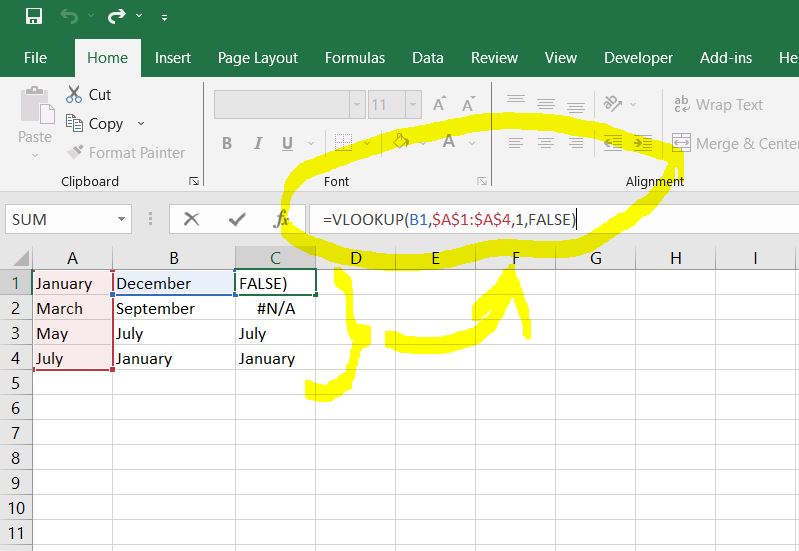
Step 2: Insert the VLOOKUP Formula
- In the first empty cell next to column B (Cell C1), type this formula:
=VLOOKUP(B1,$A$1:$A$5,1,FALSE)
The role of this formula is to search Column A for the value in Cell B1 and to return the matching value.
The ‘FALSE’ parameter means that we desire an exact match. Should you need an approximate match, you’ll have to use ‘TRUE’ instead of ‘FALSE’.
Just play around in an Excel worksheet to see how it goes.
Step 3: Drag the Formula Down
– Click and drag the corner of Cell C1 down to apply the formula to the entire column.
Step 4: Review Matches
The new column will now show the values from Column A that match Column B.
If there is no match, it will return #N/A.
Adjust the ranges in the original VLOOKUP formula as needed for your data set.
In this way, VLOOKUP allows you to easily compare two columns in Excel and identify matching values. This is a useful way to cross-check data and validate information.
Before you go:
You may also want to read this article about limiting choices in a cell to restrict data entry to a set of pre-defined values.